Shapes#
Imports#
import mumaxplus.util.shape as shapes
import numpy as np
import matplotlib.pyplot as plt
import pyvista as pv
What are Shapes?#
In mumax⁺ you can use the util package to define shapes. Each shape is a mutable instance of the Shape class, which holds and manipulates a function. This shape function takes an (x, y, z) coordinate (in meters) and returns True if it lies within the shape. All methods called upon a shape will manipulate it. They can transform, translate or rotate the shape, or can combine it with other shapes using boolean operations. There are quite a few built-in shapes.
For example, here my_shape is defined to be a basic Circle with a diameter
of 2 (meters). To check if (0, 0, 0) or (1, 1, 0) lie within it, my_shape
can be evaluated directly like a function.
my_shape = shapes.Circle(2)
print("Is (0,0,0) within my_shape?", my_shape(0,0,0))
print("Is (1,1,0) within my_shape?", my_shape(1,1,0))
Is (0,0,0) within my_shape? True
Is (1,1,0) within my_shape? False
Plotting#
We’ll need some basic code to view the shapes. To pan around in the 3D PyVista plots, you might need to install some extra stuff (namely trame):
pip install ipywidgets 'pyvista[all,trame]'
def plot_shape_2D(shape, x, y, title="", ax=None):
    """Show a shape in the xy-plane at z=0, given x and y coordinate arrays. This uses matplotlib."""
    X, Y = np.meshgrid(x, y)
    S = shape(X, Y, np.zeros_like(X))

    show_later = False
    if ax is None:
        fig, ax = plt.subplots()
        show_later = True

    dx, dy = (x[1]-x[0]), (y[1]-y[0])
    ax.imshow(S, extent=(x[0]-0.5*dx, x[-1]+0.5*dx, y[0]-0.5*dy, y[-1]+0.5*dy), origin="lower", cmap="binary")
    ax.set_xlabel("x"); ax.set_ylabel("y")
    ax.set_aspect("equal")
    if len(title) > 0: ax.set_title(title)
    if show_later: plt.show()

def plot_shape_3D(shape, x, y, z, title="", plotter=None):
    """Show a shape given x, y and z coordinate arrays. This uses PyVista."""
    X, Y, Z = np.meshgrid(x, y, z, indexing="ij")  # the logical indexing
    S = shape(X, Y, Z)
    dx, dy, dz = (x[1]-x[0]), (y[1]-y[0]), (z[1]-z[0])

                # [::-1] for [x,y,z] not [z,y,x] and +1 for cells, not points
    image_data = pv.ImageData(dimensions=(len(x)+1, len(y)+1, len(z)+1),
                spacing=(dx,dy,dz), origin=(x[0]-0.5*dx, y[0]-0.5*dy, z[0]-0.5*dz))
    image_data.cell_data["values"] = np.float32(S.flatten("F"))
    threshed = image_data.threshold_percent(0.5)  # only show True

    show_later = False
    if plotter is None:
        plotter = pv.Plotter()
        show_later = True
    plotter.add_mesh(threshed, color="white", show_edges=True, show_scalar_bar=False, smooth_shading=True)
    plotter.show_axes()
    if len(title) > 0: plotter.add_title(title)
    if show_later: plotter.show()

def plot_shape(shape, x, y, z=None, **kwargs):
    if z is None:
        return plot_shape_2D(shape, x, y, **kwargs)
    return plot_shape_3D(shape, x, y, z, **kwargs)
Built-in Shapes#
Here are a few examples of basic shapes. They can be initialized like any other instance of a class, with the approprate variables. Usually one or more diameters, not radii, are expected.
All shapes are classes in mumaxplus.util.shape, which has been imported as
shapes above. Hence, all built-in shapes can be found by
import mumaxplus.util.shape as shapes
print(dir(shapes))
['Circle', 'Cone', 'Cube', 'Cuboid', 'Cylinder', 'DelaunayHull', 'Dodecahedron', 'Ellipse', 'Ellipsoid', 'Empty', 'Icosahedron', 'Icosidodecahedron', 'ImageShape', 'Octahedron', 'Polygon', 'Rectangle', 'RegularPolygon', 'Shape', 'Sphere', 'Square', 'Tetrahedron', 'Torus', 'Universe', 'XRange', 'YRange', 'ZRange', '_Delaunay', '_Image', '_Path', '__builtins__', '__cached__', '__doc__', '__file__', '__loader__', '__name__', '__package__', '__spec__', '_np']
2D Shapes#
fig, axes = plt.subplots(2, 2, figsize=(6, 6))
x, y = np.linspace(-1, 1, 100), np.linspace(-1, 1, 100)
my_shapes = [shapes.Circle(2), shapes.Ellipse(2, 1), shapes.Rectangle(1.5, 1), shapes.RegularPolygon(7, 2)]
for shape, ax in zip(my_shapes, axes.flatten()):
    plot_shape_2D(shape, x, y, title=shape.__class__.__name__, ax=ax)
fig.tight_layout()
plt.show()
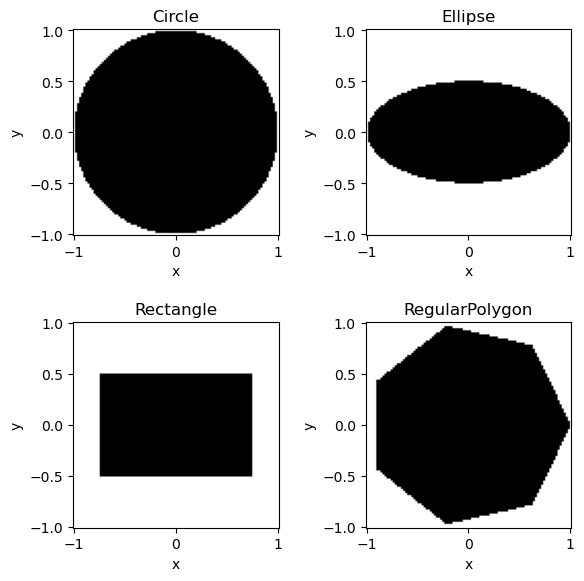
2D shapes are best defined in the xy-plane, but they exist in 3D aswell. The z-coordinate is simply ignored, so they extend indefinitely in the z-direction.
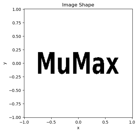
ImageShape#
A black and white image can also be used as a shape. Black is interpreted as inside (True), white as outside (False). The centers of the bottom left and top right pixels are mapped to the given x and y coordinates.
img_shape = shapes.ImageShape("shape.png", (-0.75, -0.2), (0.75, 0.2))

x = y = np.linspace(-1, 1, 256)
plot_shape(img_shape, x,y, title="Image Shape")
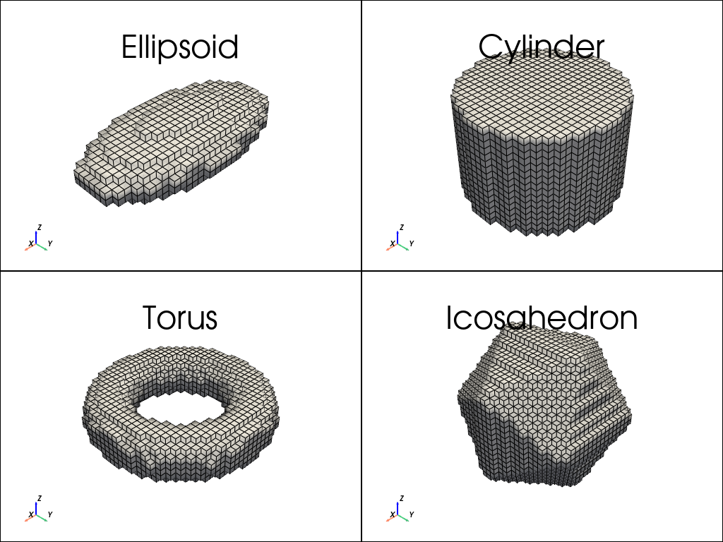
3D Shapes#
plotter = pv.Plotter(shape=(2,2))
x = y = z = np.linspace(-1, 1, 32)
my_shapes = [shapes.Ellipsoid(2, 1, 0.5), shapes.Cylinder(1.5, 1), shapes.Torus(1.5, 0.5), shapes.Icosahedron(2)]
for i, shape in enumerate(my_shapes):
    plotter.subplot(i//2, i%2)
    plot_shape_3D(shape, x, y, z, title=shape.__class__.__name__, plotter=plotter)
plotter.show()
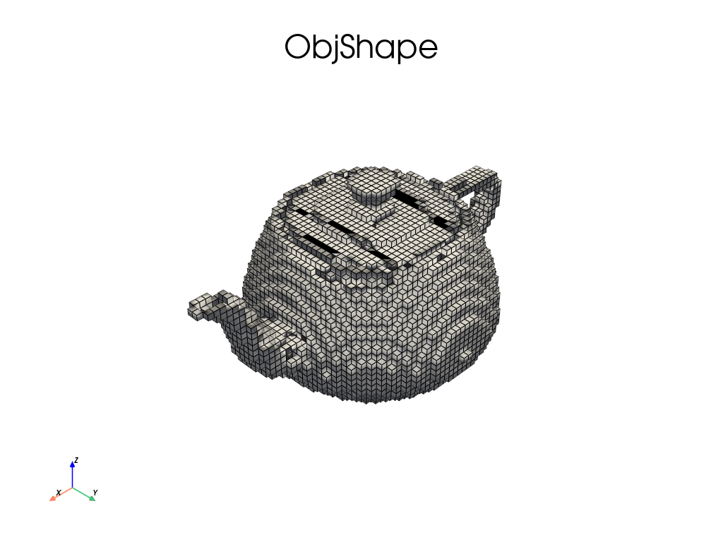
ObjShape#
A 3D object file (e.g., .obj) can also be used as a shape.
plotter = pv.Plotter()
x = y = z = np.linspace(0, 1e-7, 64)
shape = shapes.ObjShape("teapot.obj", (0, 0, 0), (1e-7, 1e-7, 1e-7), keep_aspect=True, rotate_z_up=True)
plot_shape_3D(shape, x, y, z, title=shape.__class__.__name__, plotter=plotter)
plotter.show()
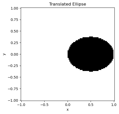
Transformations#
A shape has methods to transform it. These will modify the shape on which they are called. The simplest example is a translation.
my_ellipse = shapes.Ellipse(1, 0.75)
my_ellipse.translate_x(0.5)

x = y = z = np.linspace(-1, 1, 100)
plot_shape(my_ellipse, x, y, title="Translated Ellipse")
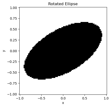
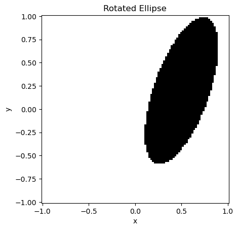
translate_y, translate_z and translate also exist. Another transformation
is the counter-clockwise rotation around a given axes in radians, such as
rotate_x, rotate_y and rotate_z.
my_ellipse = shapes.Ellipse(2, 1)
my_ellipse.rotate_z(np.pi/6)

x = y = z = np.linspace(-1, 1, 100)
plot_shape(my_ellipse, x, y, title="Rotated Ellipse")
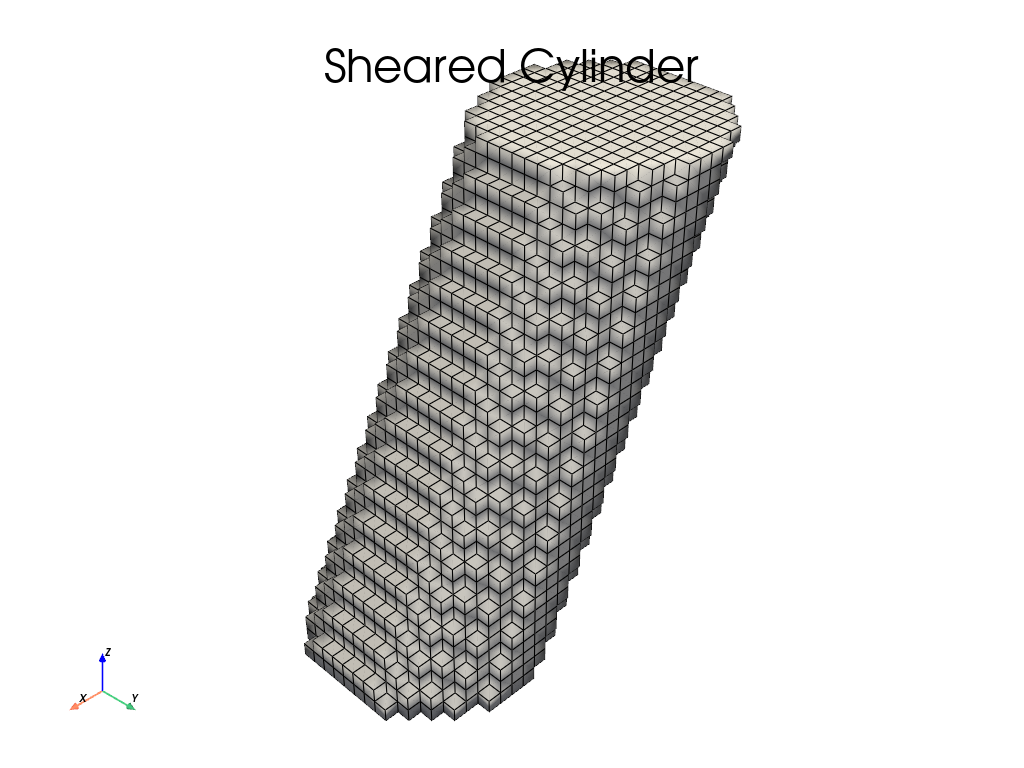
There are even more transformations, like scale, mirror and repeat, which
are fairly self-explanatory. In general a \(3 \times 3\) or even
\(4 \times 4\) transformation matrix can be passed to get any affine
transformation. As an example, here is a sheared cylinder.
Note
The inverse transformation will have to be used, as the coordinates
(x, y, z) are transformed (passive transformation) and not the shape itself
(active transformation). For example, a doubling in volume is achieved by
dividing the coordinates by two: np.diag([1/2, 1/2, 1/2]).
my_cylinder = shapes.Cylinder(1, 2)
shear_matrix = np.array([[1, 0, 0.5],
                        [0, 1, 0],
                        [0, 0, 1]])
my_cylinder.transform3(shear_matrix)

x = y = z = np.linspace(-1, 1, 32)
plot_shape(my_cylinder, x, y, z, title="Sheared Cylinder")
Multiple transformations can be chained together. This is possible because every transformation returns the shape itself. They are executed from left to right, like normal Python methods.
my_ellipse = shapes.Ellipse(1, 0.5).rotate_z(45*np.pi/180).scale(1, 2, 1).translate(0.5, 0.2, 0)

x = y = z = np.linspace(-1, 1, 100)
plot_shape(my_ellipse, x, y, title="Rotated Ellipse")
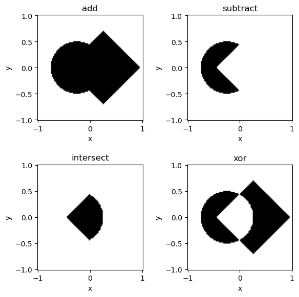
Combining Shapes#
Because every shape is a function returning a boolean (True or False), multiple shapes can be combined using boolean operations (and, or, not, xor). This is a technique called Constructive Solid Geometry (CSG).
circle = shapes.Circle(1).translate_x(-0.25)
square = shapes.Square(1).rotate_z(45*np.pi/180).translate_x(+0.25)

add = circle + square
sub = circle - square
intersect = circle & square
xor = circle ^ square

fig, axs = plt.subplots(2, 2, figsize=(6,6))

x = y = np.linspace(-1, 1, 100)
plot_shape_2D(add, x, y, title="add", ax=axs[0,0])
plot_shape_2D(sub, x, y, title="subtract", ax=axs[0,1])
plot_shape_2D(intersect, x, y, title="intersect", ax=axs[1,0])
plot_shape_2D(xor, x, y, title="xor", ax=axs[1,1])

fig.tight_layout()
plt.show()
These operations all return a new Shape instance. If you want to modify the shape
directly, you can use the methods, like add, sub, intersect and xor. You
can also use inplace operators, such as +=, -=, &= and ^=.
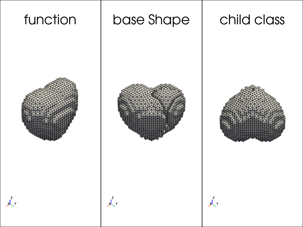
Make your own shape#
You don’t need to define a shape for the purposes of defining the geometry of a
magnet. A simple function will suffice. But if you want to take advantage of the
implemented Shape methods, that’s possible. You can use the base Shape class
and give it a function. If you want to use it more often, perhaps consider making
a new child class.
# A) a simple function
def heart_function(x,y,z):
    return (x**2 + (9/4)*(y**2) + z**2 - 1)**3 - (x**2)*(z**3) -(9/200)*(y**2)*(z**3) <= 0

# B) a base Shape class instance with a custom function
heart_shape_inst = shapes.Shape(heart_function)

# C) a Heart child class instance
class Heart(shapes.Shape):
    def __init__(self):
        super().__init__(heart_function)
heart_class_inst = Heart()


# slight transformations to keep it interesting
heart_shape_inst.rotate_z(-45*np.pi/180)
heart_class_inst.rotate_x(np.pi).rotate_z(-45*np.pi/180)

# plotting
plotter = pv.Plotter(shape=(1,3))
x = y = z = np.linspace(-1.5, 1.5, 32)
plotter.subplot(0,0)
plot_shape(heart_function, x, y, z, title="function", plotter=plotter)  # simple function
plotter.subplot(0,1)
plot_shape(heart_shape_inst, x, y, z, title="base Shape", plotter=plotter)  # base Shape instance
plotter.subplot(0,2)
plot_shape(heart_class_inst, x, y, z, title="child class", plotter=plotter)  # child Heart instance

plotter.show()
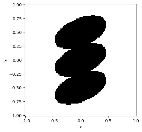
Copy#
Lastly, if you ever want to use a shape in two different ways, you can copy it
using the .copy() method.
my_shape = shapes.Ellipse(1, 0.5)
my_shape.rotate_z(np.pi/8)
top_shape = my_shape.copy().translate_y(0.5)  # translate a copy up
bottom_shape = my_shape.copy().translate_y(-0.5)  # translate a different copy down
total_shape = my_shape + top_shape + bottom_shape

x = y = np.linspace(-1, 1, 100)
plot_shape(total_shape, x, y)