Temperature

In this tutorial we show you how you can add temperature to your simulations and we compare our results with the Langevin equation.

from mumaxplus import *
import numpy as np
import matplotlib.pyplot as plt

First we define the theoretical Langevin equation.

@np.vectorize
def expectation_mz_langevin(msat, bext, temperature, cellvolume):
    kB = 1.381e-23
    xi = msat*cellvolume*bext/(kB*temperature)
    return 1/np.tanh(xi) - 1/xi

Because we want to analyse a magnet in an external field at certain temperatures, we want to have a function at hand to apply some statistics. The function will do the following:

1. Apply an external field and temperature to the magnet

2. Run a given amount of time, so the magnet can relax in the new conditions

3. Run some more, while at certain intervals the average z-magnetization is recorded

4. Return the average of the recorded z-magnetizations.

The function that does exactly this can be programmed like this:

@np.vectorize
def expectation_mz_simul(world, magnet, bext, temperature, relaxtime=1e-9, sampletime=1e-9, nsamples=200):
    world.bias_magnetic_field = (0, 0, bext)
    magnet.temperature = temperature
    world.timesolver.run(relaxtime)
    outputquantities = {"mz": lambda: magnet.magnetization.average()[2]}
    timepoints = world.timesolver.time + np.linspace(0, sampletime, nsamples)
    output = world.timesolver.solve(timepoints, outputquantities)
    return np.average(output['mz'])

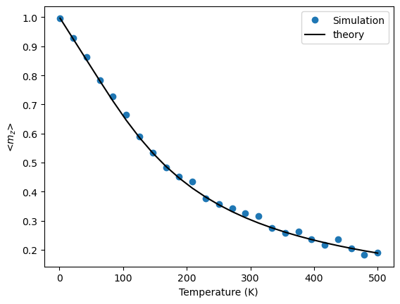
Increasing temperature

Now we will explore how the average z-magnetization of a 1D magnetic wire changes as a function of temperature while there is an external field pointing in the z-direction. We start by placing a magnet into a world.

cellvolume = 100e-27  # volume of a cubic cell
N = 1024 # number of cells

world = World(cellsize=3*[np.power(cellvolume, 1./3.)])
magnet = Ferromagnet(world, Grid((N, 1, 1)))
magnet.enable_demag = False
magnet.aex = 0.0
magnet.alpha = 0.1
magnet.msat = 800e3
magnet.magnetization = (0,0,1) # groundstate

Now we will specify the external field and the temperatures we want to examine.

bext = 0.05
temperatures = np.linspace(1, 500, 25)

We can now perform our simulation and then compare it to the theoretical result.

m_simul = expectation_mz_simul(world, magnet, bext, temperatures)
m_langevin = expectation_mz_langevin(msat, bext, temperatures, cellvolume)

plt.plot(temperatures, m_simul, 'o', label="Simulation")
plt.plot(temperatures, m_langevin, 'k-', label="theory")
plt.xlabel("Temperature (K)")
plt.ylabel("<$m_z$>")
plt.legend()
plt.show()

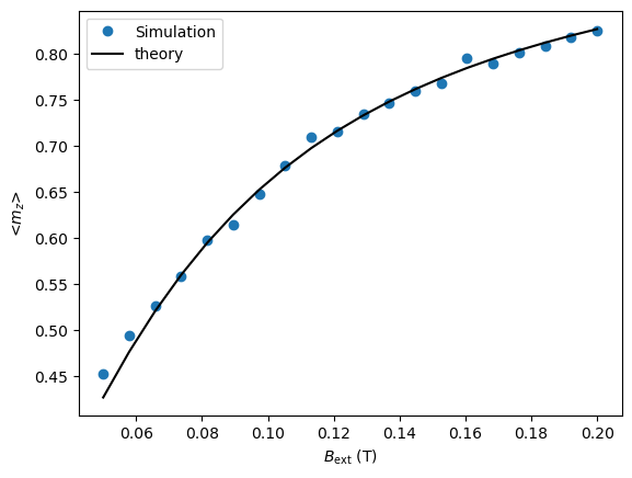
Increasing the external field

Here we will again be exploring the average z-magnetization. However, this time the external field will varry while the temperature remains constant at \(200\) K. We can use the same magnet as before, so no need to redifine the world and magnet, we can put the magnet back in its ground state and specify the temperature and external field.

magnet.magnetization = (0,0,1) # groundstate
temperature = 200
bexts = np.linspace(0.2,0.05,20)

Just like before we can now do our simulation and compare it with the theory.

m_simul = expectation_mz_simul(world, magnet, bexts, temperature)
m_langevin = expectation_mz_langevin(msat, bexts, temperature, cellvolume)

plt.plot(bexts, m_simul, 'o', label="Simulation")
plt.plot(bexts, m_langevin, 'k-', label="theory")
plt.xlabel(r"$B_{\rm ext}$ (T)")
plt.ylabel("<$m_z$>")
plt.legend()
plt.show()