mumax 3.11 examples

These are example input scripts, the full API can be found here.
A more in-depth tutorial with video recordings can be found here.

mumax³ input files are run with the command

mumax3 myfile.mx3

Output is automatically stored in the "myfile.out" directory. Additionally, a web interface provides live output. Default is http://localhost:35367.
For more details, run mumax3 -help which will show the available command-line flags (e.g. to select a certain GPU).

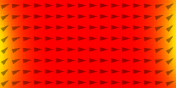
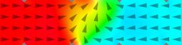
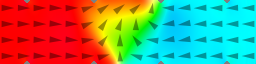
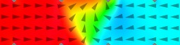
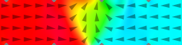
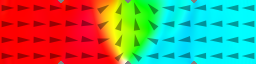
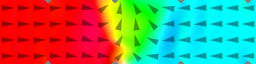
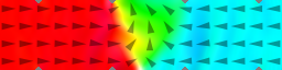
Getting started with Standard Problem #4

Let's start with the classic mumag standard problem 4, as defined here.

SetGridsize(128, 32, 1)
SetCellsize(500e-9/128, 125e-9/32, 3e-9)

Msat  = 800e3
Aex   = 13e-12
alpha = 0.02

m = uniform(1, .1, 0)
relax()
save(m)    // relaxed state

autosave(m, 200e-12)
tableautosave(10e-12)

B_ext = vector(-24.6E-3, 4.3E-3, 0)
run(1e-9)

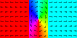
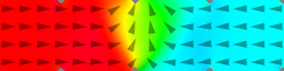
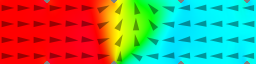
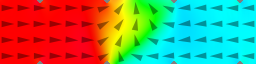
This example should be pretty straight-forward to follow. Space-dependent output is stored in OVF format, which is compatible with OOMMF and can be converted with mumax3-convert. Below is the output converted to PNG.

The data table is stored in a simple text format compatible with gnuplot, like used for the plot below.

output

Standard Problem #2

Using the scripting language explained above, relatively complex input files can be easily defined. E.g. micromagnetic standard problem #2 specifies the simulation size in exchange lengths. The script below calculates the exchange length and chooses cells not larger than 0.75 exchange lengths so that the number of cells is a power of two (for best performance).

Msat  = 1000e3
Aex   = 10e-12

// define exchange length
lex := sqrt(10e-12 / (0.5 * mu0 * pow(1000e3 ,2)))

d     := 30 * lex                        // we test for d/lex = 30
Sizex := 5*d                             // magnet size x
Sizey := 1*d
Sizez := 0.1*d

nx := pow(2, ilogb(Sizex / (0.75*lex)))  // power-of-two number of cells
ny := pow(2, ilogb(Sizey / (0.75*lex)))  // not larger than 0.75 exchange lengths

SetGridSize(nx, ny, 1)
SetCellSize(Sizex/nx, Sizey/ny, Sizez)

m = Uniform(1, 0.1, 0)                   // initial mag
relax() 

save(m)                                  // remanent magnetization
print("<m> for d/lex=30: ", m.average())

output

This example saves and prints the remanent magnetization state so we can verify it against known values.

Hysteresis

Below is an example of a hysteresis loop where we step the applied field in small increments and find the magnetization ground state after each step. Minimize() finds the ground state using the conjugate gradient method, which is very fast. However, this method might fail on very high energy initial states like a random magnetization. In that case, Relax() is more robust (albeit much slower).

SetGridsize(128, 32, 1)
SetCellsize(4e-9, 4e-9, 30e-9)

Msat  = 800e3
Aex   = 13e-12

m = randomMag()
relax()         // high-energy states best minimized by relax()


Bmax  := 100.0e-3
Bstep :=  1.0e-3
MinimizerStop = 1e-6
TableAdd(B_ext)

for B:=0.0; B<=Bmax; B+=Bstep{
    B_ext = vector(B, 0, 0)
    minimize()   // small changes best minimized by minimize()
    tablesave()
}

for B:=Bmax; B>=-Bmax; B-=Bstep{
    B_ext = vector(B, 0, 0)
    minimize()   // small changes best minimized by minimize()
    tablesave()
}

for B:=-Bmax; B<=Bmax; B+=Bstep{
    B_ext = vector(B, 0, 0)
    minimize()   // small changes best minimized by minimize()
    tablesave()
}

output

Geometry

mumax3 has powerful API to programatically define geometries. A number of primitive shapes are defined, like ellipses, rectangles, etc. They can be transformed (rotated, translated) and combined using boolean logic (add, sub, inverse). All positions are specified in meters and the origin lies in the center of the simulation box. See the full API. Edges can be smoothed to reduce staircase effects. 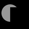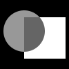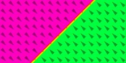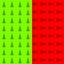EdgeSmooth=n means n³ samples per cell are used to determine its volume. EdgeSmooth=0 implies a staircase approximation, while EdgeSmooth=8 results in quite accurately resolved edges.

SetGridsize(100, 100, 50)
SetCellsize(1e-6/100, 1e-6/100, 1e-6/50)

EdgeSmooth = 8

setgeom( rect(800e-9, 500e-9) )
saveas(geom, "rect")

setgeom( cylinder(800e-9, inf) )
saveas(geom, "cylinder")

setgeom( circle(200e-9).repeat(300e-9, 400e-9, 0) )
saveas(geom, "circle_repeat")

setgeom( cylinder(800e-9, inf).inverse() )
saveas(geom, "cylinder_inverse")

setgeom( cylinder(800e-9, 600e-9).transl(200e-9, 100e-9, 0) )
saveas(geom, "cylinder_transl")

setgeom( ellipsoid(800e-9, 600e-9, 500e-9) )
saveas(geom, "ellipsoid")

setgeom( cuboid(800e-9, 600e-9, 500e-9) )
saveas(geom, "cuboid")

setgeom( cuboid(800e-9, 600e-9, 500e-9).rotz(-10*pi/180) )
saveas(geom, "cuboid_rotZ")

setgeom( layers(0, 25) )
saveas(geom, "layers")

setgeom( cell(50, 20, 0) )
saveas(geom, "cell")

setgeom( xrange(0, inf) )
saveas(geom, "xrange")

a := cylinder(600e-9, 600e-9).transl(-150e-9, 50e-9, 0 )
b := rect(600e-9, 600e-9).transl(150e-9, -50e-9, 0)

setgeom( a.add(b) )
saveas(geom, "logicAdd")

setgeom( a.sub(b) )
saveas(geom, "logicSub")

setgeom( a.intersect(b) )
saveas(geom, "logicAnd")

setgeom( a.xor(b) )
saveas(geom, "logicXor")

setgeom( imageShape("mask.png") )
saveas(geom, "imageShape")

output

Note: these are 3D geometries seen from above. The displayed cell filling is averaged along the thickness (notable in ellipse and layers example). Black means empty space, white is filled.

Initial Magnetization

Some initial magnetization functions are provided, as well as transformations similar to those on Shapes. See the Config API.

setgridsize(256, 128, 1)
setcellsize(5e-9, 5e-9, 5e-9)

m = Uniform(1, 1, 0)  // no need to normalize length
saveas(m, "uniform")

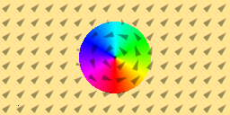
m = Vortex(1, -1)     // circulation, polarization
saveas(m, "vortex")

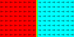
m = TwoDomain(1,0,0,  0,1,0,  -1,0,0) // Néel wall
saveas(m, "twodomain")

m = RandomMag()
saveas(m, "randommag")

m = TwoDomain(1,0,0,  0,1,0,  -1,0,0).rotz(-pi/4)
saveas(m, "twodomain_rot")

m = VortexWall(1, -1, 1, 1) 
saveas(m, "vortexwall")

m = VortexWall(1, -1, 1, 1).scale(1/2, 1, 1)
saveas(m, "vortexwall_scale")

m = Vortex(1,-1).transl(100e-9, 50e-9, 0)
saveas(m, "vortex_transl")

m = Vortex(1,-1).Add(0.1, randomMag())
saveas(m, "vortex_add_random")

m = BlochSkyrmion(1, -1).scale(3,3,1)
saveas(m, "Bloch_skyrmion")

m = NeelSkyrmion(1,-1).scale(3,3,1)
saveas(m, "Néel_skyrmion")

// set m in only a part of space, or a single cell:
m = uniform(1, 1, 1)
m.setInShape(cylinder(400e-9, 100e-9), vortex(1, -1))
m.setCell(20, 10, 0, vector(0.1, 0.1, -0.9)) // set in cell index  [20,10,0]
saveas(m, "setInShape_setCell")

//Read m from .ovf file.
m.loadfile("myfile.ovf")
saveas(m, "loadfile")

output

These initial states are approximate, after setting them it is a good idea to relax the magnetization to the actual ground state. The magnetization can also be set in separate regions, see below.

Interlude: Rotating Cheese

In this example we define a geometry that looks like a slice of cheese and have it rotate in time.

setgridsize(128, 128, 1)
setcellsize(2e-9, 2e-9, 2e-9)

d      := 200e-9
sq     := rect(d, d)                 // square with side d

h     := 50e-9
hole  := cylinder(h, h)              // circle with diameter h
hole1 := hole.transl(100e-9, 0, 0)   // translated circle #1
hole2 := hole.transl(0, -50e-9, 0)   // translated cricle #2
cheese:= sq.sub(hole1).sub(hole2)// subtract the circles from the square (makes holes).
setgeom(cheese)

msat = 600e3
aex = 12e-13
alpha = 3

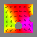
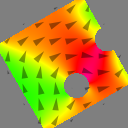
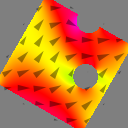
// rotate the cheese.
for i:=0; i<=90; i=i+30{
	angle := i*pi/180
	setgeom(cheese.rotz(angle))
	m = uniform(cos(angle), sin(angle), 0)
	minimize()
	save(m)
}

output

Regions: Space-dependent Parameters

Space-dependent parameters are defined using material regions. Regions are numbered 0-255 and represent different materials. Each cell can belong to only one region. At the start of a simulation all cells have region number 0.

Regions are defined with defregion(number, shape), where shape is explained in the geometry example.

When you're not using regions, like in the above examples, you'll probably set parameters with a simple assign:

Aex = 12e-13

Behind the screens, this sets Aex in all regions.

It's always a good idea to output the regions quantity, as well as all your material parameters.

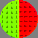
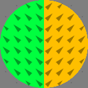
N := 128
setgridsize(N, N, 1)
c := 4e-9
setcellsize(c, c, c)

// disk with different anisotropy in left and right half
setgeom(circle(N*c))
defregion(1, xrange(0, inf))  // left half
defregion(2, xrange(-inf, 0)) // right half
save(regions)

Ku1.setregion(1, .1e6)
anisU.setRegion(1, vector(1, 0, 0))

Ku1.setregion(2, .2e6)
anisU.setRegion(2, vector(0, 1, 0))

save(Ku1)
save(anisU)

Msat = 800e3 // sets it everywhere
save(Msat)

Aex = 12e-13
alpha = 1

m.setRegion(1, uniform(1, 1, 0))
m.setRegion(2, uniform(-1, 1, 0))
saveas(m, "m_inital")
run(.1e-9)
saveas(m, "m_final")

output

Slicing and dicing output

The example below illustrates how to save only the part of the output you're interested in.

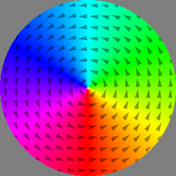
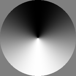
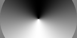
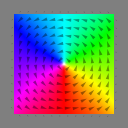
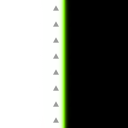
Nx := 256
Ny := 256
Nz := 1
setgridsize(Ny, Nx, Nz)
c := 4e-9
setcellsize(c, c, c)

setgeom(circle(Nx*c))

Msat  = 800e3 
Aex   = 12e-13
alpha = 1
m = vortex(1, 1)

save(m)
save(m.Comp(0))
save(Crop(m, 0, Nx/2, 0, Ny/2, 0, Nz))

mx := m.Comp(0)
mx_center := CropY(mx, Ny/4, 3*Ny/4)
save(mx_center)

output

Magnetic Force Microscopy

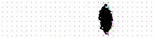
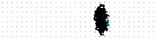
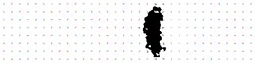
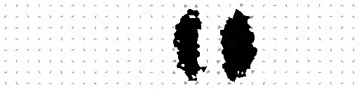
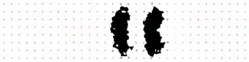
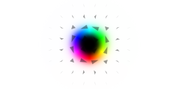
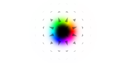
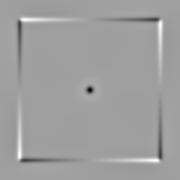
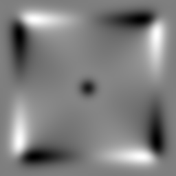
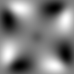
Mumax3 has built-in generation of MFM images from the magnetization. The MFM tip lift can be freely chosen. By default the tip magnetization is modeled as a point monopole at the apex. This is sufficient for most situations. Nevertheless, it is also possible to model partially magnetized tips by setting MFMDipole to the magnetized portion of the tip, in meters. E.g., if only the first 20nm of the tip is (vertically) magnetized, set MFMDipole=20e-9.

setgridsize(256, 256, 1)
setcellsize(2e-9, 2e-9, 1e-9)
setgeom(rect(400e-9, 400e-9))

msat    = 600e3
aex     = 10e-12
m       = vortex(1, 1)

relax()
save(m)

MFMLift = 10e-9
saveas(MFM, "lift_10nm")

MFMLift = 40e-9
saveas(MFM, "lift_40nm")

MFMLift = 90e-9
saveas(MFM, "lift_90nm")

output

PMA Racetrack

In this example we drive a domain wall in PMA material by spin-transfer torque. We set up a post-step function that makes the simulation box "follow" the domain wall. Like this, only a small number of cells is needed to simulate an infinitely long magnetic wire.

setGridSize(128, 128, 1)
setCellSize(2e-9, 2e-9, 1e-9)

Msat    = 600e3
Aex     = 10e-12
anisU   = vector(0, 0, 1)
Ku1     = 0.59e6
alpha   = 0.02 
Xi      = 0.2

m     = twoDomain(0, 0, 1, 1, 1, 0, 0, 0, -1) // up-down domains with wall between Bloch and Néél type
relax()

// Set post-step function that centers simulation window on domain wall.
ext_centerWall(2) // keep m[2] (= m_z) close to zero

// Schedule output
autosave(m, 100e-12)

// Run for 1ns with current through the sample
j   = vector(1.5e13, 0, 0)
pol = 1
run(.5e-9)

output

Since we center on the domain wall we can not see that it is actually moving, but the domain wall breakdown is visible.

Py Racetrack

In this example we drive a vortex wall in Permalloy by spin-transfer torque. The simulation box "follows" the domain wall. By removing surface charges at the left and right ends, we mimic an infintely long wire.

setGridSize(256, 64, 1)
setCellSize(3e-9, 3e-9, 10e-9)

Msat    = 860e3
Aex     = 13e-12
Xi      = 0.1
alpha   = 0.02 
m       = twodomain(1,0,0,  0,1,0,  -1,0,0)

notches := rect(15e-9, 15e-9).RotZ(45*pi/180).Repeat(200e-9, 64*3e-9, 0).Transl(0, 32*3e-9, 0)
setGeom(notches.inverse())

// Remove surface charges from left (mx=1) and right (mx=-1) sides to mimic infinitely long wire. We have to specify the region (0) at the boundaries.
BoundaryRegion := 0
MagLeft        := 1
MagRight       := -1
ext_rmSurfaceCharge(BoundaryRegion, MagLeft, MagRight)

relax()

ext_centerWall(0) // keep m[0] (m_x) close to zero

// Schedule output
autosave(m, 50e-12)
tableadd(ext_dwpos)   // domain wall position
tableautosave(10e-12)

// Run the simulation with current through the sample
pol = 0.56
J   = vector(-10e12, 0, 0)
Run(0.5e-9)

output

Since we center on the domain wall we can not really see the motion, despite the vortex wall moving pretty fast. Note the absence of closure domains at the edges due to the surface charges being removed there.

Voronoi tessellation

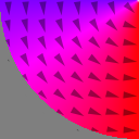
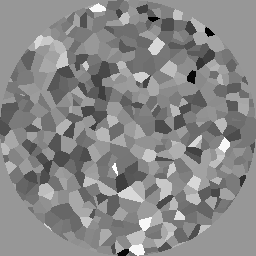
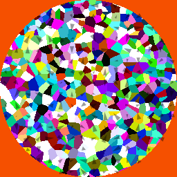
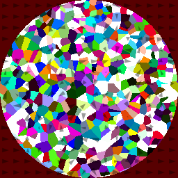
In this example we use regions to specify grains in a material. The built-in extension ext_makegrains is used to define grain-like regions using Voronoi tessellation. We vary the material parameters in each grain.

N := 256
c := 4e-9
d := 40e-9
setgridsize(N, N, 1)
setcellsize(c, c, d)

setGeom(circle(N*c))

// define grains with region number 0-255
grainSize  := 40e-9  // m
randomSeed := 1234567
maxRegion  := 255
ext_makegrains(grainSize, maxRegion, randomSeed)

defregion(256, circle(N*c).inverse()) // region 256 is outside, not really needed

alpha = 3
Kc1   = 1000
Aex   = 13e-12
Msat  = 860e3

// set random parameters per region
for i:=0; i<maxRegion; i++{
	// random cubic anisotropy direction
	axis1  := vector(randNorm(), randNorm(), randNorm())
	helper := vector(randNorm(), randNorm(), randNorm())
	axis2  := axis1.cross(helper)  // perpendicular to axis1
	AnisC1.SetRegion(i, axis1)     // axes need not be normalized
	AnisC2.SetRegion(i, axis2)

	// random 10% anisotropy variation
	K := 1e5
	Kc1.SetRegion(i, K + randNorm() * 0.1 * K)
}

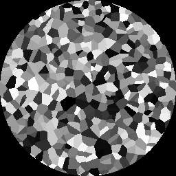
// reduce exchange coupling between grains by 10%
for i:=0; i<maxRegion; i++{
	for j:=i+1; j<maxRegion; j++{
		ext_ScaleExchange(i, j, 0.9)
	}
}

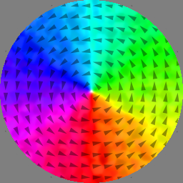
m = vortex(1, 1)
run(.1e-9)

save(regions)
save(Kc1)
save(AnisC1)
save(AnisC2)
save(m)
save(exchCoupling)

output

RKKY

Scaling the exchange coupling between regions can be used to obtain antiferromagnetic coupling like the RKKY interaction. In that case we only model the magnetic layers and do not explicitly add a spacer layer (which is negligibly thin). We scale the exchange coupling to get the desired RKKY strength: scale = (RKKY * cellsize_z) / (2 * Aex).

N := 10
setgridsize(N, N, 2)

c := 1e-9
setcellsize(c, c, c)

defRegion(0, layer(0))
defRegion(1, layer(1))

Msat = 1e6

Aex  = 10e-12
RKKY := -1e-3 // 1mJ/m2
scale := (RKKY * c) / (2 * Aex.Average())
ext_scaleExchange(0, 1, scale)

tableAdd(E_total)

m.setRegion(0, uniform(1, 0, 0))

for ang:=0; ang<360; ang++{
	m.setRegion(1, uniform(cos(ang*pi/180), sin(ang*pi/180), 0))	
	t = ang * 1e-9 // output "time" is really angle
	tablesave()
}

output

Slonczewski STT

Example of a spin-torque MRAM stack consisting of a fixed layer, spacer and free layer. Only the free layer magnetization is explicitly modeled, so we use a 2D grid. The fixed layer polarization is set with FixedLayer = ..., which can be space-dependent. The spacer layer properties are modeled by setting the parameters Lambda and EpsilonPrime. Finally Pol sets the current polarization and J the current density, which should be along z in this case. Below we switch an MRAM bit.

// geometry
sizeX := 160e-9
sizeY := 80e-9
sizeZ := 5e-9

Nx := 64
Ny := 32
 
setgridsize(Nx, Ny, 1)
setcellsize(sizeX/Nx, sizeY/Ny, sizeZ)
setGeom(ellipse(sizeX, sizeY))

// set up free layer
Msat  = 800e3
Aex   = 13e-12
alpha = 0.01
m     = uniform(1, 0, 0)

// set up spacer layer parameters
lambda       = 1
Pol          = 0.5669
epsilonprime = 0

// set up fixed layer polarization
angle := 20
px := cos(angle * pi/180)
py := sin(angle * pi/180)
fixedlayer = vector(px, py, 0)

// send current
Jtot := -0.008            // total current in A
area := sizeX*sizeY*pi/4
jc   := Jtot / area       // current density in A/m2
J = vector(0, 0, jc)

// schedule output & run
autosave(m, 100e-12)
tableautosave(10e-12)
run(1e-9)

output

Spinning hard disk

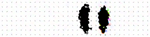
Using the Shift function, we can shift the system (magnetization, regions and geometry) by a given number of cells. Here we use this feature to simulate a moving hard disk platter. A time-dependent gaussian field profile mimics the write field.

Nx := 512
Ny := 128
c := 5e-9
setgridsize(Nx, Ny, 1)
setcellsize(c, c, c)

ext_makegrains(30e-9, 256, 0)

// PMA material
Ku1   = 0.4e6
Aex   = 10e-12
Msat  = 600e3
alpha = 1

delta := 0.2 // anisotropy variation

for i:=0; i<256; i++{
	// random cubic anisotropy direction
	AnisU.SetRegion(i, vector(delta*(rand()-0.5), delta*(rand()-0.5), 1))

	// strongly reduce exchange coupling between grains
	for j:=i+1; j<256; j++{
		ext_scaleExchange(i, j, 0.1)
	}
}

m = uniform(0, 0, 1)

// Gaussian external field profile
mask := newVectorMask(Nx, Ny, 1)
for i:=0; i<Nx; i++{
	for j:=0; j<Ny; j++{
		r := index2coord(i, j, 0)
		x := r.X()
		y := r.Y()
		Bz := exp(-pow((x-500e-9)/100e-9, 2)) * exp(-pow(y/250e-9, 2))
		mask.setVector(i, j, 0, vector(0, 0, Bz))
	}
}

// 500Mbit/s oscillating write field
f := 0.5e9
A := 1.5
B_ext.add(mask, -A*sin(2*pi*f*t))

autosave(m, 600e-12)

// Spin the hard disk
ShiftMagR = vector(0, 0, 1) // new magnetization to enter
for i:=0; i<120; i++{
	run(30e-12)
	Shift(-1) // one cell to the left
}